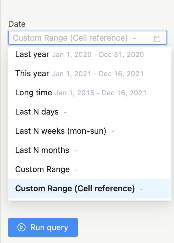
When selecting a date range, there’s a choice in Two Minute Reports called “Custom Range (cell reference)”. You may use this feature if you prefer to use a date range from a spreadsheet cell. It allows you to fetch data from your Data Sources for any data range that you’d like.
In this example, the Facebook report has a start date of 11//17/2021 and an end date of 12/15/2021, which are populated in cells. Those cells are F6 and H6.
Using the Custom Range (cell reference) date range selection, your queries can pick up the date range dynamically from your Spreadsheet. So whenever a query runs, the new date ranges from your Spreadsheet will be picked up and used to filter your data.
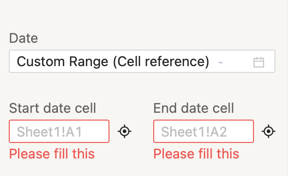
Once you choose the Custom Range from the Date Range drop down, you can enter spreadsheet formulas in the Start Date Cell and End Date Cell text box. The left side of the explanation point is the name of the sheet tab while the right side is the actual cell.
If your sheet is named Facebook Report and the start date is on F6, enter Facebook Report’!F6 under the Start date cell. Likewise if the end date is H6, enter Facebook Report’!H6.
Two Minute reports allows you to fetch data from your Data Sources for any data range that you’d like. For that we have a preset list of Date Ranges that you can select from in your Query.
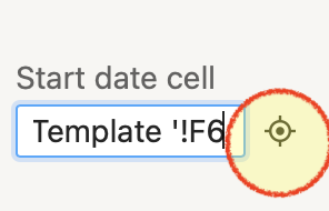
If you prefer to do this automatically, you can also click on the Reference Picker (crosshair icon) to pick up the cell reference.
Steps:
- Highlight the cell that contains the date.
- Click the Reference Picker (cross-hair icon)
- Wait for 3 seconds to auto-populate the field.
This way you can quickly change your date ranges for your queries directly from your Spreadsheets.
We hope you liked this tutorial on dynamic date ranges. If you have any questions please feel free to contact our Support Team. Also check our pages on our schedule refresh feature, Google Sheets templates, etc. You may also check out other articles in our knowledge base on how to use Two Minute Reports in Google Sheets


